Activities (MAST)
MAST is the Maryland Activity Scheduling and Travel model, the activity model of MILES.
At a glance
| Engine | MAST, Java, built on the ABIT code base |
| Code | activity/ (coefficients, run scripts, Java source) |
| Estimated on | 2017/18 Regional Travel Survey, estimation half |
| Models | 3,946 survey distributions, 13 location and tour-formation logits, 7 mode-choice models |
| Sensitive to | Car and transit times and costs, parking, zone attributes, household composition, cars and licences |
| Produces | One weekday plan per person: activities, locations, times, modes |
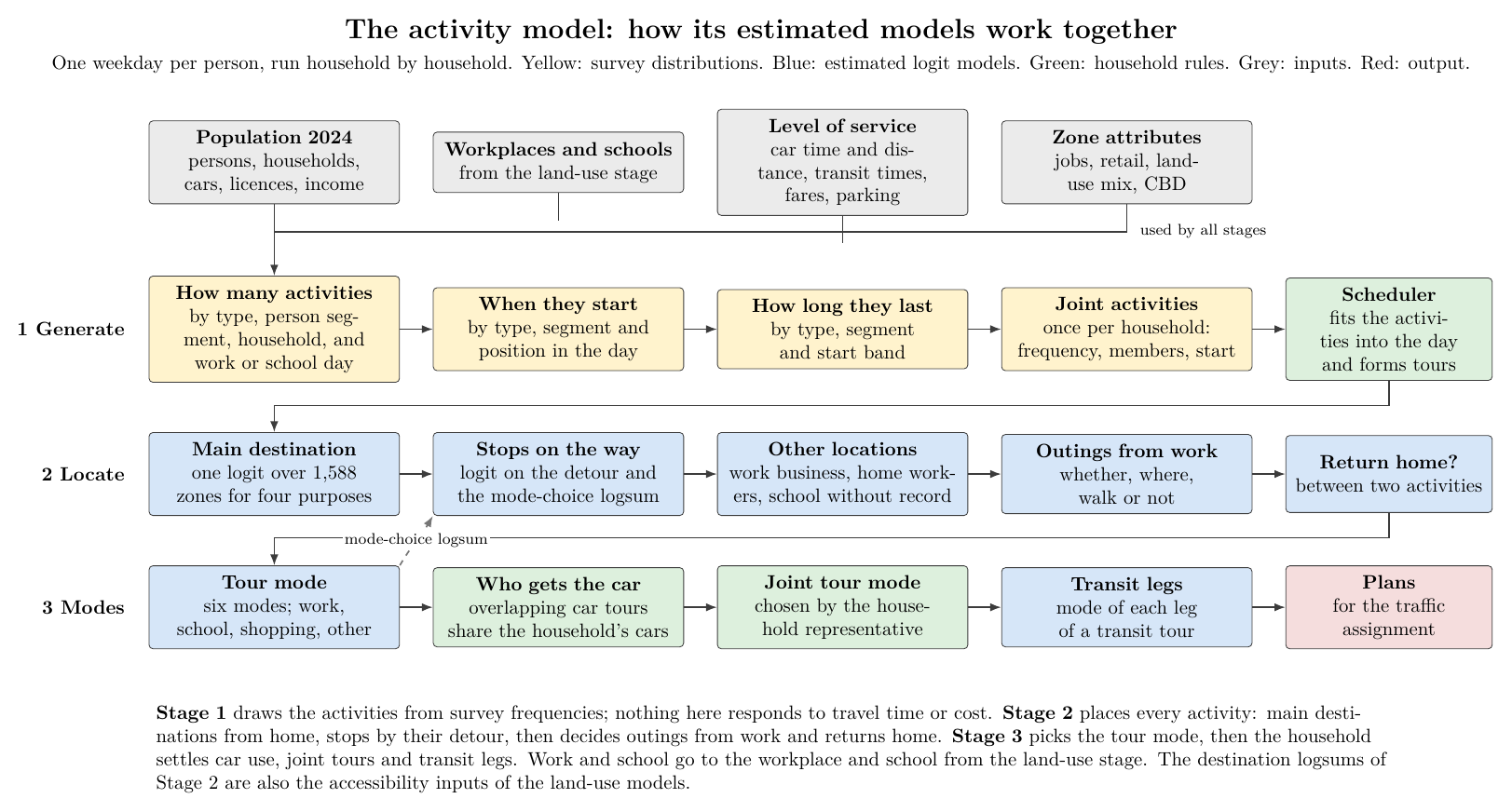
MAST generates, schedules and locates the activity episodes of every person for one weekday and assigns their tour modes. Work and school episodes go to the job and school the person holds in the land-use model; every other episode is located by an estimated model. All distributions and parameters come from the estimation half of the travel survey, and no calibration factor is applied.
Lineage
MAST is built on the code base of the ABIT activity-based model of the Maryland set-up and adopts the scheduling idea of TASHA. Against the original set-up it changes the following:
| Part | What it does |
|---|---|
| TASHA-type generation and scheduling | Episodes drawn from the survey's joint distributions of frequency, start time and duration; scheduled by precedence; household joint activities |
| Conditioning on the day | Frequencies depend on whether a work or school episode is scheduled that day |
| Licence split | Shopping, recreation, accompanying and other frequencies of persons 16+ split by driving licence |
| Joint activities by work or school | Joint frequency, membership and start time depend on the members' work or school that day |
| Pooled primary destination model | One logit for four purposes with purpose scales, over all 1,588 zones |
| Attraction terms | One attraction variable per location model, as its own log term, with ln zone area |
| Stop models | Stops located by their detour and the mode-choice logsum |
| Outings from the workplace | Whether, where and by which mode |
| Return-home model | Whether a person goes home between two out-of-home episodes |
| Re-estimated tour mode models | Time and cost, paid parking, children, stops; four segments |
| Household car allocation | Overlapping car-driver tours share the household's cars |
| Joint-tour representative | Joint tours take the mode chosen by a household representative with a group-level model |
| Transit leg modes | Mode of each leg of a transit tour |
Stage 1: generation and scheduling
The number of episodes \(n\), the arrival time \(t\) and the duration \(\delta\) of each person and episode type are drawn from
| Symbol | Meaning |
|---|---|
| \(\tau\) | episode type (13, below) |
| \(g\) | person segment (10): worker with a usual workplace, working at home, without a fixed workplace; elementary, middle, high-school and post-secondary student; non-worker; retiree; child under 5 |
| \(h\) | household class (3): single person, several persons without children, with a child under 16 |
| \(m\) | whether a work or school episode is scheduled that day |
| \(r\) | number of episodes of higher precedence on the day (0, 1, 2+) |
| \(e\) | episode index (1, 2, 3+) |
| \(\sigma\) | schedule attribute |
| \(\beta_t\) | start band |
Episode types, in order of scheduling precedence
| Code | Episode type |
|---|---|
| WB | Work business: a work episode away from the usual workplace |
| WAHB | Work trip of a person whose usual workplace is home |
| PW | Primary work: at the usual workplace, arriving before 15:00 |
| SW | Secondary work: at the usual workplace, arriving at 15:00 or later |
| RHW | Return home from work (for example, lunch at home) |
| SCH | School, college or daycare |
| JO_REC, JO_OTH | Joint recreation, joint other activity with household members |
| JS | Joint shopping |
| IO_REC, IO_ACC, IO_OTH | Individual recreation, accompanying (drop-off or pick-up), other errand |
| IS | Individual shopping |
The 3,946 distributions are weighted relative frequencies of the estimation half; when a cell is too thin, the model falls back to a coarser cell. Start times are in 15-minute bins; durations in 5-minute bins up to two hours, then 15-minute bins. Joint episodes are generated once per household, by household composition, workers and whether members work or attend school that day.
Whether a worker has a usual workplace, works at home or has no fixed workplace is drawn from the survey shares by age band. Frequencies, start times and durations come from survey distributions and therefore do not respond to travel time or cost.
The scheduler inserts episodes into the day in precedence order, shifts and shortens them to fit, and forms home-based tours.
Stage 2: locations and tours
Main destination of discretionary tours
The main activity of each discretionary tour is located from home with one multinomial logit over the 1,588 zones, for four purposes (shopping, recreation, accompanying, other errands), estimated jointly with a scale \(\mu_p\) per purpose:
\(x_{pj}\) is the one attraction variable of the purpose (retail jobs; school enrolment for accompanying), entered as its own log term. \(f\) is a piecewise-linear car distance with knots at 1, 2, 5, 10, 20 and 50 km, \(GT_{hj}\) the car generalised time, \(\mathbf z_j\) zone attributes (intrazonal, ln zone area, land-use mix, high job density, Baltimore City, the District, other states, county and state boundaries) and \(\mathbf w_n\) person, household, time-of-day and tour flags interacting with log distance. The mode-choice logsum was tested as the impedance and lost to car time for every purpose. Estimated on 14,341 tours (62 parameters).
Stops
Intermediate stops are located in time order by their detour between the previous location \(a\) and the next anchor \(b\) (the main activity on the way out, home on the way back):
where \(LS\) is the logsum of the tour mode-choice model of the stop's purpose. One model per stop purpose: shopping, recreation, accompanying and other errands. As in the main destination model, each has one attraction variable as a log term (retail jobs for shopping, school enrolment for accompanying).
Other locations
Logits of the same form locate work business (workers with a usual workplace; other persons), the work trips of persons who work at home (office jobs as attraction), and school and daycare episodes of persons without a school record (one pooled model, school enrolment as attraction).
Outings and returns home
- Outing from the workplace (binary logit): whether a work episode contains an outing, from work duration, arrival time, a CBD workplace and the home–work distance. A location logit places its first stop, and a binary logit with 7 parameters decides whether it is walked or keeps the mode of the work tour.
- Return home (binary logit): for every pair of consecutive out-of-home episodes, whether the person goes home in between, from the detour via home, the distance from home, the episode types, person and household variables (including fewer cars than drivers) and the time of day; 33 parameters.
Stage 3: modes
Tour mode choice
The main mode of each home-based tour is chosen after its destination, timing and stops are known. Six modes (car driver as reference, car passenger, bus, train, walk, bicycle) and four segments (work, school, shopping, other):
| Segment | Time and cost | Structure |
|---|---|---|
| Work | Generalised cost \(GC = T + 60\,C/VOT\), with \(VOT = 0.5 \times\) hourly household income | MNL, weighted to ACS commute shares (WESML) |
| School | Not significant; distance only | MNL |
| Shopping | Separate time and cost (VOT $12.3/h) | MNL |
| Other | Separate time and cost (VOT $41.2/h) | Nested: car driver with car passenger, bus with train |
\(\mathbf z_n\) holds person, household and area-type variables, the paid-parking share at the destination and whether the tour has stops; \(d_n\) is the round-trip car distance. On work tours a dollar is worth 2.96 minutes for a household with an income of $84,216. The tour models have no term for fewer cars than drivers, because cars are allocated in the household stage. Race is not used in any MAST model.
Household stage
- Cars: car-driver tours whose times away from home overlap beyond the household's cars form a conflict set; the cars go to the feasible combination with the highest household utility, and a tour without a car takes its next-best mode.
- Joint tours: a household representative (the oldest member who can drive, otherwise the oldest member) chooses the mode with a group-level model for joint shopping and for joint recreation and other tours; when the representative drives, the other members ride as car passengers.
- Transit legs: a multinomial logit with 35 parameters gives the mode of each leg of a transit tour (transit, walk, car passenger, car driver, bicycle). Car driver is available only when a household car is free over the tour window, the rule under which the model was estimated. The model keeps a term for fewer cars than drivers, because the car allocation covers only part of that effect.
Output
One weekday plan per person: the sequence of activities with their zone, start and end times, and the mode of each trip. These plans are converted to MATSim plans for the assignment (assignment).